Objective

Have the regional flows in Barrow in Furness changed?

Data

Data are sourced from Census 2011 and Census 2021 flows data.

Approach

Geocode location
Identify the OA / LSOA / MSOA of interest
Compare commuting flows

Barrow-in-Furness

Code

## Geocode the Location
library(tidygeocoder)
lnglat <- dplyr::tibble(location = "Barrow Shipyard") |>
  geocode(location, method = "osm")

Passing 1 address to the Nominatim single address geocoder

Query completed in: 1 seconds

Geocode the Location

Code

## Plot on a Map
library(leaflet)
leaflet(lnglat) |>
  addTiles() |>
  addPopups(lng = ~long, lat = ~lat, popup = "Barrow-in-Furness")

Generate a Bounding Box based on Defined Distance

Code

## Create a Circle
spdf <- sf::st_as_sf(lnglat, coords = c("long", "lat"), crs = 4326)
spdf |>
  sf::st_transform(27700) |>
  sf::st_buffer(5e3) |>
  sf::st_transform(4326) |>
  leaflet::leaflet() |> 
  leaflet::addTiles() |>
  leaflet::addPolygons()

Query the Output Areas within that Bounding Box

Code

# Load the MSOA in the Area
db <- DBI::dbConnect(
    RPostgres::Postgres(),
    db = "census", 
    host = "localhost", 
    port = 5432,
    user = "postgres", 
    password = Sys.getenv("postgre_pw")
  )

bbox <- spdf |>
  sf::st_transform(27700) |>
  sf::st_buffer(2.5e3) |>
 # sf::st_transform(4326) |>
  sf::st_bbox()

query_bounding_box <- function(bbox, tbl = "ew_msoa_2021", srid = 27700){
  
glue::glue("SELECT * FROM {tbl}
  WHERE  geometry 
  && 
    ST_MakeEnvelope (
      {bbox[1]}, {bbox[2]}, 
      {bbox[3]}, {bbox[4]}, 
      {srid})")
}

oa_2021 <- sf::st_read(db, query = query_bounding_box(bbox, "ew_oa_2021")) |> sf::st_transform(4326)

oa_2011 <- sf::st_read(db, query = query_bounding_box(bbox, "infuse_oa_lyr_2011")) |> sf::st_transform(4326)

leaflet(oa_2021) |>
  leaflet::addTiles() |>
  leaflet::addPolygons()

Code

leaflet(oa_2011) |>
  leaflet::addTiles() |>
  leaflet::addPolygons()

Extract the Census Flow Data for Those Output Areas

Code

oa21cd_f <- oa_2021 |>
  dplyr::as_tibble() |>
  dplyr::pull(oa21cd) |>
  unique()

oa11cd_f <- oa_2011 |>
  dplyr::as_tibble() |>
  dplyr::pull(geo_code) |>
  unique()


flow_2021 <- db |>
  dplyr::tbl("ODWP01EW_OA") |>
  dplyr::filter(`oa_of_workplace_code` %in% oa21cd_f) |>
  dplyr::collect()

flow_2011 <- db |>
  dplyr::tbl("WF03UK_oa_v1") |>
  dplyr::filter(area_of_workplace %in% oa11cd_f) |>
  dplyr::collect() |>
  dplyr::filter(stringr::str_detect(area_of_usual_residence, "^E|^W"))

Calculate the Distance Between Work Areas

Code

oa11_work <- paste0("'", flow_2011$area_of_workplace |> unique() |> paste(collapse = "','"), "'")

oa11_work_geo <- sf::st_read(
  db, query = glue::glue(
    "SELECT * FROM infuse_oa_lyr_2011 WHERE geo_code IN ({oa11_work})"
  )
) |>
  sf::st_transform(4326) |>
  sf::st_centroid() |>
  dplyr::select(oa11cd_work = geo_code, work_geo = geometry)

Warning: st_centroid assumes attributes are constant over geometries

Code

oa11_residence <-  paste0("'", flow_2011$area_of_usual_residence |> unique() |> paste(collapse = "','"), "'")

oa11_residence_geo <-  sf::st_read(
  db, query = glue::glue(
    "SELECT * FROM infuse_oa_lyr_2011 WHERE geo_code IN ({oa11_residence})"
  )
) |>
  sf::st_transform(4326) |>
  sf::st_centroid() |>
  dplyr::select(oa11cd_residence = geo_code, residence_geo = geometry)

Warning: st_centroid assumes attributes are constant over geometries

Code

flow_2011_geo <- flow_2011 |>
  dplyr::select(
    oa11cd_residence = area_of_usual_residence,
    oa11cd_work = area_of_workplace, 
    count = persons) |>
  dplyr::left_join(oa11_residence_geo) |>
  dplyr::left_join(oa11_work_geo)  |>
  dplyr::mutate(
    dist = sf::st_distance(residence_geo, work_geo, by_element = TRUE)
    )

Joining with `by = join_by(oa11cd_residence)`
Joining with `by = join_by(oa11cd_work)`

Code

oa21_work <- paste0("'",flow_2021$oa_of_workplace_code |> unique() |>
  paste(collapse = "','"), "'")

oa21_work_geo <- sf::st_read(
  db, query = glue::glue(
    "SELECT * FROM ew_oa_2021 WHERE oa21cd IN ({oa21_work})"
    )) |>
  sf::st_transform(4326) |>
  sf::st_centroid() |>
  dplyr::select(oa21cd_work = oa21cd, work_geo = geometry)

Warning: st_centroid assumes attributes are constant over geometries

Code

oa21_residence <- paste0("'",flow_2021$output_areas_code |> unique() |>
  paste(collapse = "','"), "'")

oa21_residence_geo <- sf::st_read(
  db, query = glue::glue(
    "SELECT * FROM ew_oa_2021 WHERE oa21cd IN ({oa21_residence})"
    )) |>
  sf::st_transform(4326) |>
  sf::st_centroid() |>
  dplyr::select(oa21cd_residence = oa21cd, residence_geo = geometry)

Warning: st_centroid assumes attributes are constant over geometries

Code

flow_2021_geo <- flow_2021 |>
  dplyr::select(
    oa21cd_residence = output_areas_code,
    oa21cd_work = oa_of_workplace_code, 
    workplace_indicator = place_of_work_indicator_4_categories_label,
    count) |>
  dplyr::left_join(oa21_residence_geo) |>
  dplyr::left_join(oa21_work_geo)  |>
  dplyr::mutate(
    dist = sf::st_distance(residence_geo, work_geo, by_element = TRUE)
    )

Joining with `by = join_by(oa21cd_residence)`
Joining with `by = join_by(oa21cd_work)`

Compare Summary Statistics

Code

flow_2011_geo |>
  dplyr::summarise(avg = mean(dist),
                   total = sum(count*dist),
                   w_avg = sum(count*dist)/sum(count),
                   count = sum(count)) |>
  dplyr::mutate(year = 2011) |>
  dplyr::bind_rows(
    
  flow_2021_geo |>
    dplyr::summarise(avg = mean(dist),
                     total = sum(count*dist),
                     w_avg = sum(count*dist)/sum(count),
                     count = sum(count)) |>
    dplyr::mutate(year = 2021)
  )

# A tibble: 2 × 5
     avg      total  w_avg count  year
     [m]        [m]    [m] <dbl> <dbl>
1 15862. 199680118.  8565. 23313  2011
2 23047. 247641474. 10045. 24653  2021

Code

dist_2011 <- flow_2011_geo |>
  dplyr::select(count, dist) |>
  purrr::pmap(function(count, dist) rep(dist, count)) |>
  unlist()

dist_2021 <- flow_2021_geo |>
  dplyr::select(count, dist) |>
  purrr::pmap(function(count, dist) rep(dist, count)) |>
  unlist()

flow_2021_geo |>
  dplyr::group_by(workplace_indicator) |>
  dplyr::summarise(count = sum(count))

# A tibble: 2 × 2
  workplace_indicator                               count
  <chr>                                             <dbl>
1 Mainly working at or from home, No fixed place     6105
2 Working in the UK but not working at or from home 18548

Code

dist_2021_not_wfh <- flow_2021_geo |>
  dplyr::filter(workplace_indicator != "Mainly working at or from home, No fixed place") |>
  dplyr::select(count, dist) |>
  purrr::pmap(function(count, dist) rep(dist, count)) |>
  unlist()

distances <- dplyr::tibble(year = as.character(2011), dist = dist_2011) |>
  dplyr::bind_rows(
    dplyr::tibble(year = as.character(2021), dist = dist_2021)
  ) |>
  dplyr::bind_rows(
    dplyr::tibble(year = "2021 (Not WfH)", dist = dist_2021_not_wfh)
  )

library(ggplot2)

ggplot(distances) + geom_density(aes(dist, colour = as.factor(year)))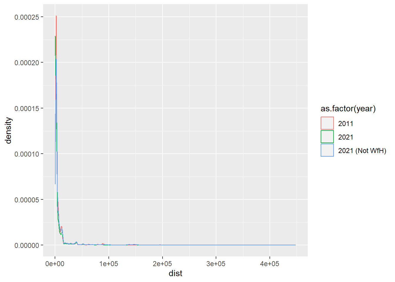

Code

distances |>
  dplyr::group_by(year) |>
  dplyr::summarise(
    min = min(dist),
    p25 = quantile(dist, 0.25),
    p50 = quantile(dist, 0.5),
    p75 = quantile(dist, 0.75),
    p80 = quantile(dist, 0.8),
    p90 = quantile(dist, 0.9),
    p95 = quantile(dist, 0.95),
    max = max(dist),
    mean = mean(dist),
    count = dplyr::n()
  )

# A tibble: 3 × 11
  year             min   p25   p50   p75   p80    p90    p95    max   mean count
  <chr>          <dbl> <dbl> <dbl> <dbl> <dbl>  <dbl>  <dbl>  <dbl>  <dbl> <int>
1 2011               0 1390. 2358. 5493. 7189. 12860. 37939. 4.48e5  8565. 23313
2 2021               0    0  1869. 4583. 6482. 13821. 41820. 4.26e5 10045. 24653
3 2021 (Not WfH)     0 1528. 2676. 7069. 9700. 25459. 64253. 4.26e5 13351. 18548

Code

f <- flow_2021_geo$oa21cd_residence
flow_2021_geo |>
  dplyr::mutate(dist = as.numeric(dist)) |>
  dplyr::filter(dist >300000) |>
  dplyr::left_join(
    db |>
    dplyr::tbl("oa21_lsoa21_msoa21_lad22") |>
      dplyr::filter(oa21cd %in% f) |>
      dplyr::collect() |>
    dplyr::select(oa21cd, lsoa21nm),
    by = c("oa21cd_residence" = "oa21cd")
  ) |>
  dplyr::select(oa21cd_residence,lsoa21nm, dist, count) |>
  dplyr::arrange(-dist) |>
  head(20)

# A tibble: 20 × 4
   oa21cd_residence lsoa21nm                                    dist count
   <chr>            <chr>                                      <dbl> <dbl>
 1 E00102181        South Hams 011A                          426161.     1
 2 E00172060        Plymouth 026E                            420302.     1
 3 E00076025        Plymouth 026B                            419614.     1
 4 E00076642        Plymouth 020D                            418097.     1
 5 E00102098        South Hams 002C                          416306.     1
 6 E00076190        Plymouth 006C                            415347.     1
 7 E00076617        Plymouth 001D                            412426.     1
 8 E00076615        Plymouth 001D                            412346.     3
 9 E00160124        Arun 012B                                405904.     1
10 E00186746        Tonbridge and Malling 014H               400118.     1
11 E00086244        Portsmouth 015B                          395814.     1
12 E00086490        Portsmouth 022C                          395804.     1
13 E00086497        Portsmouth 022C                          395768.     1
14 E00086276        Portsmouth 012D                          395599.     1
15 E00086230        Portsmouth 012D                          395430.     1
16 E00116021        Gosport 008C                             394082.     1
17 E00180417        Isle of Wight 002D                       393534.     1
18 E00115933        Gosport 003B                             391535.     1
19 E00115547        Fareham 003C                             386220.     1
20 E00077504        Bournemouth, Christchurch and Poole 017B 385595.     1

Code

top20_2021 <- flow_2021_geo |>
  dplyr::left_join(
    db |>
  dplyr::tbl("oa21_lsoa21_msoa21_lad22") |>
  dplyr::select(oa21cd, lad22nm) |>
  dplyr::collect(),
  by = c("oa21cd_residence" = "oa21cd")
  ) |>
  dplyr::group_by(lad22nm) |>
  dplyr::summarise(count = sum(count)) |>
  dplyr::arrange(-count) |>
  head(20) |>
  dplyr::mutate(year = 2021) |>
  dplyr::rename(lad = lad22nm) |>
  head(20)

top20_2011 <- flow_2011_geo |>
  dplyr::left_join(
    db |>
    dplyr::tbl("oa11_lsoa11_msoa11_lad_2017") |>
    dplyr::select(OA11CD, LAD17NM) |>
    dplyr::distinct() |>
    dplyr::collect(),
    by = c("oa11cd_residence" = "OA11CD")
  ) |>
  dplyr::group_by(LAD17NM) |>
  dplyr::summarise(count = sum(count)) |>
  dplyr::arrange(-count) |>
  dplyr::mutate(year = 2011) |>
  dplyr::rename(lad= LAD17NM) |>
  head(20)

  ggplot(top20_2021) + geom_bar(aes(factor(lad,rev(unique(lad))), count), stat = "identity") + facet_wrap(~year) +
  coord_flip()

Code

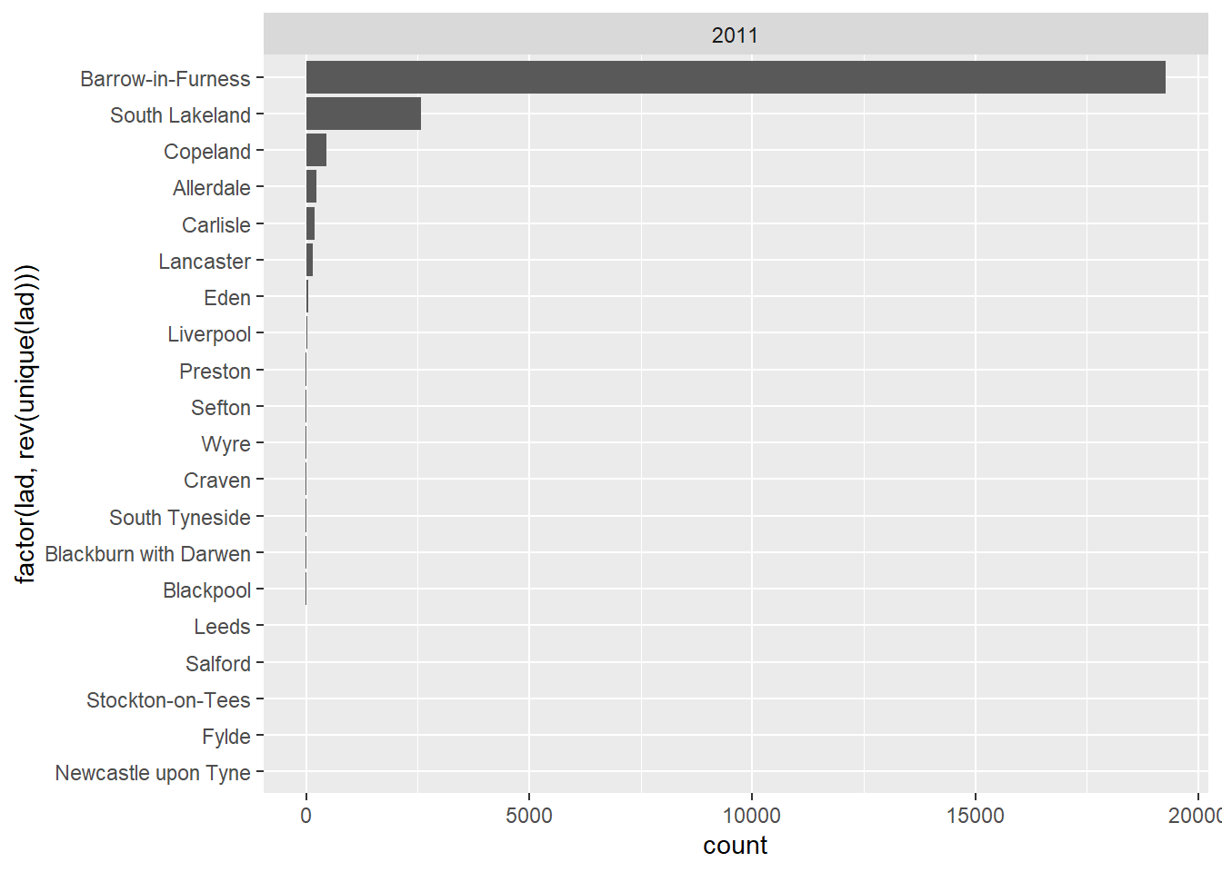
  ggplot(top20_2011) + geom_bar(aes(factor(lad,rev(unique(lad))), count), stat = "identity") + facet_wrap(~year) +
  coord_flip()